Hands-on: implement a spatial transformer network by yourself

Spatial transformer networks understand how to rotate, translate a image. How does it learn to do it?

Intro

Spatial Transformer Networks is a paper published by Max Jaderberg, Karen Simonyan, Andrew Zisserman and Koray Kavukcuoglu at 2015, at the moment of writing, it has been cited 3715 times.

The full code implementing the STN concept is available on GitHub: https://github.com/xeonqq/spatial_transformer_network

The network works like a plug and play enhancement NN module to your exisiting neural network. It can perform affine transformation to the input image in order to ensure the inputs to the classification network to be spatial invariant.

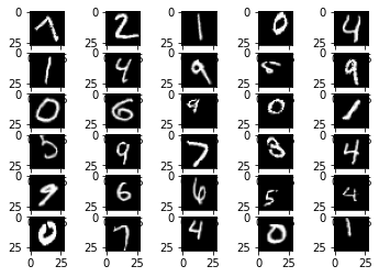
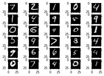
The figure below shows how a STN can transform an affine distorted MNIST dataset into a “corrected” one:

Why spatial invariant is important and what does that mean?

Let’s look at the following examples using this online hand-written digit recognition tool trained with MNIST dataset.

First we draw a normal 2, it has been recognized correctly, second we draw a rotated 2, it’s recognized as 8:

One might say, because the network is not trained with such rotated inputs, therefore the network fails to recognize in this case.

To verify it, I build a simple network with two fully connected layer same as the google tutorial. Then I trained this network with both original MNIST dataset and affine distorted MNIST dataset mixed together. The accuracy when evaluating the original MNIST is still good, with accuracy of 0.9767. However, when evaluating with distorted MNIST, the accuracy has only 0.8388. In this case, we can say this fully connected layer based model architecture is not spatial invariant, because it fails to classify the images when they are affine transformed (scale, rotate, translation, etc).

Well, how about CNN with max-pooling layers. Because I hear from here that max-pooling layers help to remove spatial variance.

Talking is cheap, let also experiment a CNN with distorted MNIST dataset. Below is the construction of the CNN, with 2 conv layers + 2 max pooling layers + 3 fully connected layers:

model = tf.keras.models.Sequential([
  tf.keras.layers.Conv2D(6, (3,3), input_shape=(28, 28, 1),padding='valid',activation="relu"),
  tf.keras.layers.MaxPooling2D((2, 2)),
  tf.keras.layers.Conv2D(16, (3,3),padding='valid',activation="relu"),
  tf.keras.layers.MaxPooling2D((2, 2)),
  tf.keras.layers.Flatten(),
  tf.keras.layers.Dense(120, activation='relu'),
  tf.keras.layers.Dense(84, activation='relu'),
  tf.keras.layers.Dense(10),
])

After training with the same mixed dataset as before, we have an accuracy of 0.9872 for the original MNIST dataset and 0.9367 for the distorted MNIST dataset! That’s already a lot of improvement. Therefore, it is right indeed that max-pooling layer helps to remove the spatial variance of the input.

Can we do better by using STN

In this post, we will see how Spatial Transformer Networks can allievate spatial variance problem, and how to implement the STN concept using keras from tensorflow 2. We will also cover many important details during implementation. The goal is to reach compariable accuary like using the orignal MNIST dataset, without modifying the CNN classification network.

Dataset Preparation

For this project we create our own distorted MNIST dataset with the help of imgaug. imgaug is an opensource tool (included in my docker), which can easily perform affine transformations to images. We use MNIST as the basis, for each image we will randomly apply one of the following transformation:

scale [0.5, 1.3] (unit percentage)
rotation [-60, 60] (unit degree)
shear [-40, 40] (unit degree)
scale [0.6, 1.1] then translation [-0.2, 0.2] (unit percentage)
scale [0.6, 1.1], translation [-0.2, 0.2], rotation [-30, 30] then shear [-15, 15].

After applying the distortion, we place original MNIST (left), distorted MNIST (right) for comparision:

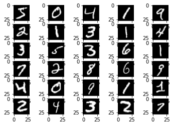
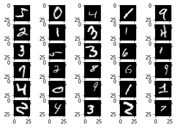
For detail of using imgaug, refer to my implementation

Implementation

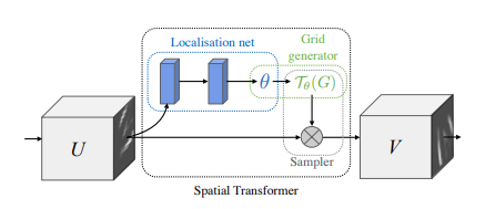
The Spatial Transformer Networks consists of the following key components: stn

Localization net: it can be a CNN or fully connectly NN, as long as the last layer of it is a regression layer, and it will generate 6 numbers representing the affine transformation θ.
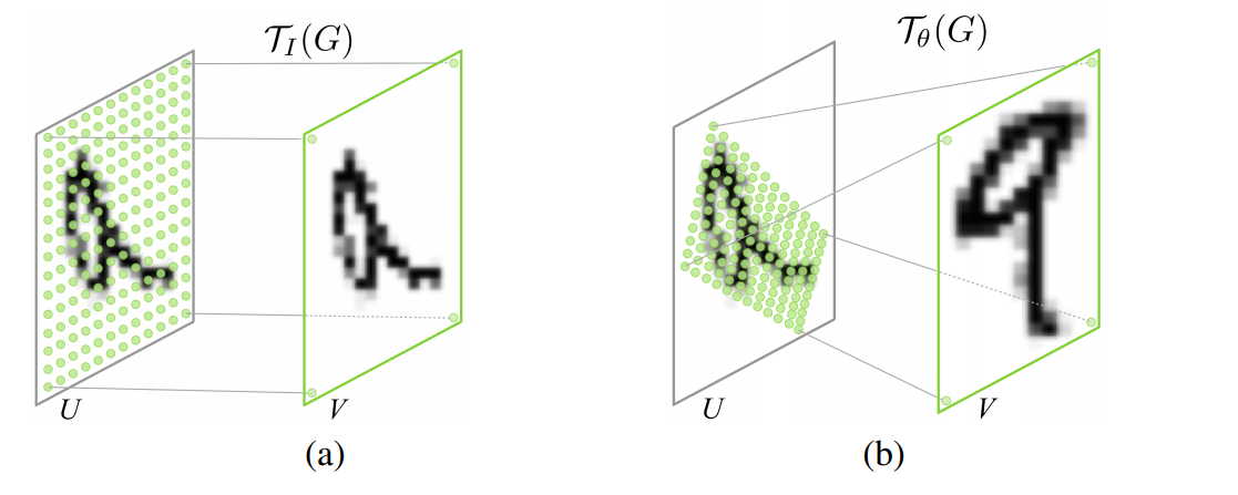
Grid Generator: it first generates a grid over the target image V, each point of the grid just corresponds to the pixel coordinate of each pixel in the target image. Secondly, it uses the transformation θ to transform the grid.
Sampler: The transformed grid is like a mask over the source image U, which retrieve the pixels under the mask. However, the transformed grid no longer contains integer values, therefore a bilinear interpolation is performed on the source image U, in order to get an estimated pixel value under the transformed grid.

Localization Net

The localization net takes the input images of dimension [batch_size, height, width, channels] and produces transformation for each input image of dimension. The transformations will be of dimension [batch_size, 6]. Here we use a CNN architecture which is very similar to our classification network, execpt some special setup on the last layer.

def create_localization_head(inputs):
    x = Conv2D(14, (5,5),padding='valid',activation="relu")(inputs)
    x = MaxPooling2D((2, 2), strides=2)(x)
    x = Conv2D(32, (5,5), padding='valid',activation="relu")(x)
    x = MaxPooling2D((2, 2),strides=2)(x)
    x = Flatten()(x)    
    x = Dense(120, activation='relu')(x)
    x = Dropout(0.2)(x)
    x = Dense(84, activation='relu')(x)
    x = Dense(6, activation="linear", kernel_initializer="zeros",
              bias_initializer=lambda shape, dtype: tf.constant([1,0,0,0,1,0], dtype=dtype))(x) # 6 elements to describe the transformation
    return tf.keras.Model(inputs, x)

In order to make the last layer a regression layer, I didn’t use ReLu as activation function, but simply use linear, to not constrain the output.

Implementation detail: Note biases are initialized with the identity transformation. Without this manual bias initialization, the network tend to rotate all the images to a fix angle which may not fit the human preference.

Grid Generator

In the Grid Generator, one must note the transformation θ is applied on the grid generated from the target image V instead of the source image U, and it is called inverse mapping in the world of image processing. On the other hand if we transform the source image U to the target image V, this process is called forward mapping.

The forward mapping iterates over each pixel of the input image, computes new coordinates for it, and copies its value to the new location. But the new coordinates may not lie within the bounds of the output image and may not be integers. The former problem is easily solved by checking the computed coordinates before copying pixel values. The second problem is solved by assigning the nearest integers to x′ and y′ and using these as the output coordinates of the transformed pixel. The problem is that each output pixel may be addressed several times or not at all (the latter case leads to “holes” where no value is assigned to a pixel in the output image).

The inverse mapping iterates over each pixel of the output image and uses the inverse transformation to determine the position in the input image from which a value must be sampled. In this case the determined positions also may not lie within the bounds of the input image and may not be integers. But the output image has no holes Uni Auckland

After understanding the inverse mapping, let me show the implementation details:

def generate_normalized_homo_meshgrids(inputs):
    # for x, y in grid, -1 <=x,y<=1
    batch_size = tf.shape(inputs)[0]
    _, H, W,_ = inputs.shape
    x_range = tf.range(W)
    y_range = tf.range(H) 
    x_mesh, y_mesh = tf.meshgrid(x_range, y_range)
    x_mesh = (x_mesh/W-0.5)*2
    y_mesh = (y_mesh/H-0.5)*2
    y_mesh = tf.reshape(y_mesh, (*y_mesh.shape,1))
    x_mesh = tf.reshape(x_mesh, (*x_mesh.shape,1))
    ones_mesh = tf.ones_like(x_mesh)
    homogeneous_grid = tf.concat([x_mesh, y_mesh, ones_mesh],-1)
    homogeneous_grid = tf.reshape(homogeneous_grid, (-1, 3,1))
    homogeneous_grid = tf.dtypes.cast(homogeneous_grid, tf.float32)
    homogeneous_grid = tf.expand_dims(homogeneous_grid, 0)
    return tf.tile(homogeneous_grid, [batch_size, 1,1,1])

In generate_normalized_homo_meshgrids function, given the input dimension, we can generate a meshgrid. The mesh grid is then normalized between [-1, 1), so that the rotation or translation will be performed relative to the center of the image. Each grid is also extended with a third dimenstion, filled with ones, hence the name homogeneous_grid. It is to perform the transformation more convienient in the following transform_grids.

def transform_grids(transformations, grids, inputs):
    trans_matrices=tf.reshape(transformations, (-1, 2,3))
    batch_size = tf.shape(trans_matrices)[0]
    gs = tf.squeeze(grids, -1)
    reprojected_grids = tf.matmul(trans_matrices, gs, transpose_b=True)
    # transform grid range from [-1,1) to the range of [0,1)
    reprojected_grids = (tf.linalg.matrix_transpose(reprojected_grids) + 1)*0.5
    _, H, W, _ = inputs.shape
    reprojected_grids = tf.math.multiply(reprojected_grids, [W, H])
    return reprojected_grids

In transform_grids we apply the transformations generated from the localization net onto the grids from generate_normalized_homo_meshgrids to get the reprojected_grids. After transformation, the reprojected_grids are rescaled back to be in the range of width and height of the input image.

Implementation detail: Note the batch_size needs to be retrieved via tf.shape function instead of simple inputs.shape, because batch_size is a dynamic shape, which can be None at model initialization.

Sampler

def generate_four_neighbors_from_reprojection(inputs, reprojected_grids):
    _, H, W, _ = inputs.shape
    x, y = tf.split(reprojected_grids, 2, axis=-1)
    x1 = tf.floor(x)
    x1 = tf.dtypes.cast(x1, tf.int32)
    x2 = x1 + tf.constant(1) 
    y1 = tf.floor(y)
    y1 = tf.dtypes.cast(y1, tf.int32)
    y2 = y1 + tf.constant(1) 
    y_max = tf.constant(H - 1, dtype=tf.int32)
    x_max = tf.constant(W - 1, dtype=tf.int32)
    zero = tf.zeros([1], dtype=tf.int32)
    x1_safe = tf.clip_by_value(x1, zero, x_max)
    y1_safe = tf.clip_by_value(y1, zero, y_max)
    x2_safe = tf.clip_by_value(x2, zero, x_max)
    y2_safe = tf.clip_by_value(y2, zero, y_max)
    return x1_safe, y1_safe, x2_safe, y2_safe

def bilinear_sample(inputs, reprojected_grids):
    x1, y1, x2, y2 = generate_four_neighbors_from_reprojection(inputs, reprojected_grids)
    x1y1 = tf.concat([y1,x1],-1)
    x1y2 = tf.concat([y2,x1],-1)
    x2y1 = tf.concat([y1,x2],-1)
    x2y2 = tf.concat([y2,x2],-1)
    pixel_x1y1 = tf.gather_nd(inputs, x1y1, batch_dims=1)
    pixel_x1y2 = tf.gather_nd(inputs, x1y2, batch_dims=1)
    pixel_x2y1 = tf.gather_nd(inputs, x2y1, batch_dims=1)
    pixel_x2y2 = tf.gather_nd(inputs, x2y2, batch_dims=1)
    x, y = tf.split(reprojected_grids, 2, axis=-1)
    wx = tf.concat([tf.dtypes.cast(x2, tf.float32) - x, x -tf.dtypes.cast(x1, tf.float32)],-1)
    wx = tf.expand_dims(wx, -2)
    wy = tf.concat([tf.dtypes.cast(y2, tf.float32) - y, y - tf.dtypes.cast(y1, tf.float32)],-1)
    wy = tf.expand_dims(wy, -1)
    Q = tf.concat([pixel_x1y1, pixel_x1y2, pixel_x2y1, pixel_x2y2], -1)
    Q_shape = tf.shape(Q)
    Q = tf.reshape(Q, (Q_shape[0], Q_shape[1],2,2))
    Q = tf.cast(Q, tf.float32)

    r = wx@Q@wy
    _, H, W, channels = inputs.shape
    r = tf.reshape(r, (-1,H,W,1))
    return r

bilinear

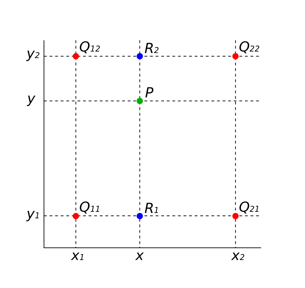
bilinear_sample first use generate_four_neighbors_from_reprojection to get the 4 nearest neighbors for each reprojected grid point. The Q matrix is constructed using the four points. Then by using the linear interpolation formular from Wikipedia, the pixel value at the projection point is estimated.

Implementation detail: Since python >= 3.5 the @ operator is supported (see PEP 465). In TensorFlow, it simply calls the tf.matmul()

Put Everything Together

def spatial_transform_input(inputs, transformations):
    grids = generate_normalized_homo_meshgrids(inputs)
    reprojected_grids = transform_grids(transformations, grids,inputs)
    result = bilinear_sample(inputs, reprojected_grids)
    return result

inputs = Input(shape=(H,W,1))
localization_head= create_localization_head(inputs)
x = spatial_transform_input(inputs, localization_head.output)
x = model(x)
st = tf.keras.Model(inputs, x)
loss_fn = tf.keras.losses.SparseCategoricalCrossentropy(from_logits=True)
st.compile(optimizer="adam",
              loss=loss_fn,
              metrics=['accuracy'])

Implementation detail: tf.keras.Model takes two parameters, first input, second output (in this case x). This is the trick how we combine STN with exsiting CNN together.

Evaluation

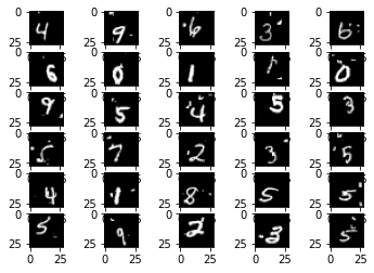
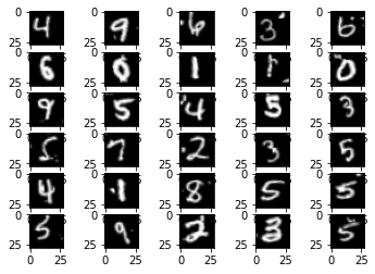
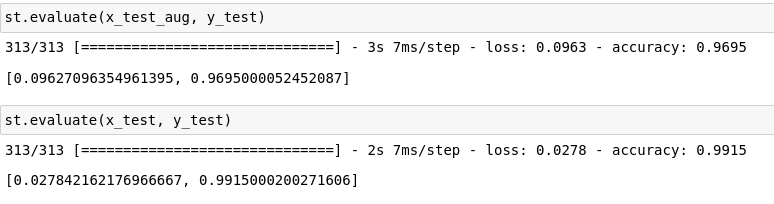eval Afer training the STN with the mixed dataset (distorted MNIST + orignal_MNIST), we can get accuracy 0.97 for the distorted MNIST, and 0.99 for the original MNIST. So STN does improve the performance of our model. Let’s have a look of the STN transformed input for the CNN: (input images (left), transformed input images (right)):